Stepping into Footwear Market with Web Scraping

The footwear market is one of the most quickly growing fashion apparel markets and it can be easily understood through a bit of web scraping. The web is full of public footwear product data that we can take advantage of for free using Python and web scraping libraries.

In this overview, we'll do a demonstration of product performance analytics through web scraping. We'll be scraping Goat.com - one of the most popular footwear marketplaces and making sense of it using Python and Jupyter Notebooks. This short demonstration will give you a taste of what you can do with web scraping and data analytics.

Project Setup

We'll be using basic Jupyter notebooks. If you're unfamiliar with Jupyter it's a great tool for data analysis and visualization. You can learn more about it jupyter.org.

Our setup for this article we'll be very simple and we'll be using the basic Python libraries:

• pandas as our data analysis library
• matplotlib as our data visualization library
• ipywidgets as our interactive widgets library for customizing data visualization interactively

All of these can be installed using pip console command:

$ pip install notebook pandas matplotlib ipywidgets

All resources used in this article can be found on our Kaggle directory:

• Notebook with all of the code used in this article.
• Air Jordan 3 Dataset used in this article.

Footwear Market Sources

We've covered the scraping of many fashion websites that cover footwear products like:

How to Scrape StockX e-commerce Data with Python

StockX is an online marketplace for buying and selling authentic sneakers, streetwear, watches, and designer handbags. The most interesting part about StockX is that it treats apparel items as a commodity and tracks their value over time

How to Scrape Vestiaire Collective for Fashion Product Data

Vestiaire Collective is a luxury fashion resale platform from France. It's a popular web scraping target as it's one of the biggest second-hand markets for luxury fashion items.

How to Scrape Fashionphile for Second Hand Fashion Data

Fashionphile is a popular online platform for second-hand luxury fashion items. It is known for careful product curation making it ideal for web scraping second hand luxury fashion items as data quality is particularly high.

How to Scrape Nordstrom Fashion Product Data

Nordstrom is a leading fashion retailer based in US with an equally popular e-commerce store that operates worldwide. It's a popular web scraping target because of the rich data it offers and its position in the fashion industry.

How to Scrape Goat.com for Fashion Apparel Data in Python

Goat.com is an up-and-coming global apparel platform covering the newest and second-hand fashion items. Goat is known for having an enormous product dataset that is constantly updated and easy to scrape.

Scraping Dataset

For this tutorial, we'll be using Goat.com data as it's especially popular when it comes to footwear products.

For our example dataset we'll focus on a single footwear product "Air Jordan 3" which can be scraped using using Goat.com scraper.

Note we're using Scrapfly SDK to scrape our dataset quickly without being blocked as Goat.com is using Cloudflare Bot Management to block web scraping. ScrapFly SDK allows easy anti scraping protection bypass which will allow us to quickly scrape Goat.com without being blocked:

import asyncio
import json
import math
from datetime import datetime
from pathlib import Path
from typing import Dict, List, Optional
from urllib.parse import quote, urlencode
from uuid import uuid4

from scrapfly import ScrapeApiResponse, ScrapeConfig, ScrapflyClient

scrapfly = ScrapflyClient(key="YOUR SCRAPFLY KEY")


def find_hidden_data(result: ScrapeApiResponse) -> dict:
    """extract hidden NEXT_DATA from page html"""
    data = result.selector.css("script#__NEXT_DATA__::text").get()
    data = json.loads(data)
    return data


async def scrape_products(urls: List[str]) -> List[dict]:
    """scrape a single goat.com product page for product data"""
    to_scrape = [ScrapeConfig(url=url, cache=True, asp=True) for url in urls]
    products = []
    async for result in scrapfly.concurrent_scrape(to_scrape):
        try:
            data = find_hidden_data(result)
            product = data["props"]["pageProps"]["productTemplate"]
            product["offers"] = data["props"]["pageProps"]["offers"]["offerData"]
            products.append(product)
        except Exception as e:
            print(f"Failed to scrape {result.context['url']}; got {e}")
    return products


async def scrape_search(query: str, max_pages: Optional[int] = 10) -> List[Dict]:
    def make_page_url(page: int = 1):
        params = {
            "c": "ciojs-client-2.29.12",  # this is hardcoded API version
            "key": "key_XT7bjdbvjgECO5d8",  # API key which is hardcoded in the client
            "i": str(uuid4()),  # unique id for each request, generated by UUID4
            "s": "2",
            "page": page,
            "num_results_per_page": "24",
            "sort_by": "relevance",
            "sort_order": "descending",
            "fmt_options[hidden_fields]": "gp_lowest_price_cents_3",
            "fmt_options[hidden_fields]": "gp_instant_ship_lowest_price_cents_3",
            "fmt_options[hidden_facets]": "gp_lowest_price_cents_3",
            "fmt_options[hidden_facets]": "gp_instant_ship_lowest_price_cents_3",
            "_dt": int(datetime.utcnow().timestamp() * 1000),  # current timestamp in milliseconds
        }
        return f"https://ac.cnstrc.com/search/{quote(query)}?{urlencode(params)}"

    url_first_page = make_page_url(page=1)
    print(f"scraping product search paging {url_first_page}")
    # scrape first page
    result_first_page = await scrapfly.async_scrape(ScrapeConfig(url=url_first_page, asp=True))
    first_page = json.loads(result_first_page.content)["response"]
    results = [result["data"] for result in first_page["results"]]

    # find total page count
    total_pages = math.ceil(first_page["total_num_results"] / 24)
    if max_pages and max_pages < total_pages:
        total_pages = max_pages

    # scrape remaining pages
    print(f"scraping remaining total pages: {total_pages-1} concurrently")
    to_scrape = [ScrapeConfig(make_page_url(page=page), asp=True) for page in range(2, total_pages + 1)]
    async for result in scrapfly.concurrent_scrape(to_scrape):
        data = json.loads(result.content)
        items = [result["data"] for result in data["response"]["results"]]
        results.extend(items)

    return results

To gather our dataset we can use the following scrape code:

# Scraper code from
# https://scrapfly.io/blog/how-to-scrape-goat-com-fashion-apparel/#full-scraper-code
import json
from pathlib import Path

async def scrape_all_search(query):
    search = await scrape_search(query, max_pages=30)
    product_urls = [f"https://www.goat.com/{item['product_type']}/{item['slug']}" for item in search]
    search_products = await scrape_products(product_urls)
    Path(f"{query}.json").write_text(json.dumps(search_products, indent=2, ensure_ascii=False))

asyncio.run(scrape_all_search("Air Jordan 3"))

This will yield over 600 footwear products that are variations of "Air Jordan 3" sneakers. This dataset can also be found on our kaggle directory

Let's see what we can learn from this dataset.

Market Distribution

Market distribution is some of the easiest data analytics we can do that'll give us an overview of the market. We can analyze the market distribution by product colors, designers and other product features. Let's do just that!

To start with our data analysis let's load our dataset into a Pandas DataFrame:

import pandas as pd
import matplotlib.pyplot as plt

data = pd.read_json('air-jordan-3.json')
# convert datetime string to datetime object
data['releaseDate'] = pd.to_datetime(data['releaseDate'])
# convert price strings to floats
for _, row in data.iterrows():
    for size_obj in row['offers']:
        size_obj = float(size_obj['price'])
data.head()

This will give us a DataFrame with over 600 product rows and many data field columns like price, color, release date etc.

Now we can start analyzing our data. Let's start with a basic question:

What colors do Air Jordan 3's come in?

# Color distribution by percentage
color_counts = data['color'].value_counts().head(10)
color_percentages = (color_counts / color_counts.sum()) * 100
ax = color_counts.plot(kind='bar', title='Top 10 Most Common Shoe Colors', figsize=(10, 6))
for i, p in enumerate(ax.patches):
    ax.annotate(f"{color_percentages[i]:.1f}%", (p.get_x() + p.get_width() / 2., p.get_height()),
                 ha='center', va='baseline', fontsize=10, color='black', xytext=(0, 5),
                 textcoords='offset points')
plt.xlabel('Color')
plt.ylabel('Shoe count')
plt.show()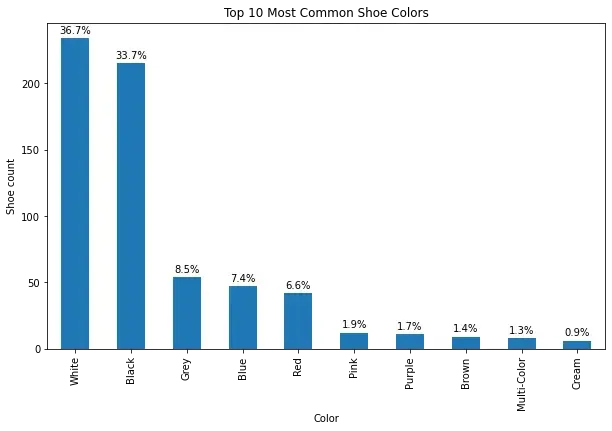

Here we see the color distribution of Jordai Air 3's available on Goat.com. White and Black seem to be the most common colors by far.

Next, we can take a peek at which Jordan Air 3 designer is the most popular:

designer_counts = data['designer'].value_counts().head(10)
designer_counts_perc = (designer_counts / designer_counts.sum()) * 100
ax = designer_counts.plot(kind='bar', title='Top 10 Shoe Designers by Number of Shoes Designed', figsize=(10, 6))
for i, p in enumerate(ax.patches):
    ax.annotate(f"{designer_counts_perc[i]:.1f}%", (p.get_x() + p.get_width() / 2., p.get_height()),
                 ha='center', va='baseline', fontsize=10, color='black', xytext=(0, 5),
                 textcoords='offset points')
plt.xlabel('Designer')
plt.ylabel('Number of Shoes Designed')
plt.show()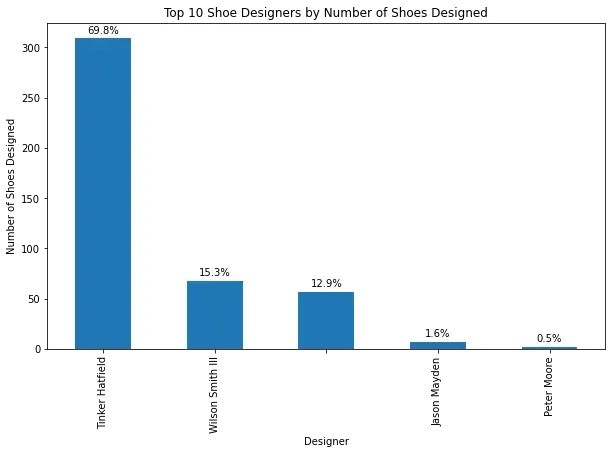

Here we can see that Tinker Hatfield's Jordan Air 3's are by far the most popular versions of this particular sneaker.

Distribution analysis is a great way to get a quick overview of the market. We can also use this data to create a simple recommendation system that'll recommend products based on the user's preferences.

Price Distribution

The most attractive data field is of course the price. We can do a fair bit of price based analytics which can be applied in product reselling or even flipping between many different storefronts.

Since our Goat.com dataset contains pricing based on footwear size, color and other feature we can figure out which products have highest demand. For example - the average price per shoe size:

sizes_list = []
prices_list = []

for _, row in data.iterrows():
    for size_obj in row['offers']:
        if not(6 < size_obj['size'] < 16):  # only men sized shoes
            continue
        sizes_list.append(size_obj['size'])
        prices_list.append(float(size_obj['price']))

size_price_df = pd.DataFrame({'size': sizes_list, 'price': prices_list})
average_price_by_size = size_price_df.groupby('size')['price'].mean().sort_values(ascending=False)

# Create the bar chart
average_price_by_size.plot(kind='bar', figsize=(10, 6))
plt.title('Average Price per Shoe Size')
plt.xlabel('Shoe Size')
plt.ylabel('Average Price')
plt.show()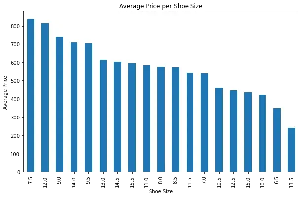

Here we can see that price distribution is fairly chaotic though with clear indicators that smallest sizes 6.5 and 7 being the cheapest.

We can take this even further and see how the price distribution changes based on the color of the shoe. Let's add an slider widget to display the average price per shoe color for a given shoe size:

import ipywidgets as widgets
from IPython.display import display

def plot_avg_price_by_color(shoe_size):
    colors_list = []
    prices_list = []

    for _, row in data.iterrows():
        for size_obj in row['offers']:
            if size_obj['size'] != shoe_size:
                continue
            colors_list.append(row['color'])
            prices_list.append(float(size_obj['price']))

    color_price_df = pd.DataFrame({'color': colors_list, 'price': prices_list})
    average_price_by_color = color_price_df.groupby('color')['price'].median().sort_values(ascending=False)

    # Create the bar chart
    average_price_by_color.plot(kind='bar', figsize=(10, 6))
    plt.title(f'Average Price per Shoe Color for size {shoe_size}')
    plt.xlabel('Shoe Color')
    plt.ylabel('Average Price')
    plt.ylim(0, 4000)
    plt.show()

# Create slider widget
shoe_size_slider = widgets.FloatSlider(value=6, min=6, max=14, step=0.5, description='Shoe Size:')
widgets.interact(plot_avg_price_by_color, shoe_size=shoe_size_slider)

Here we can see how ipywidgets can be effortlessly used to create interactive visualizations based on customized inputs. We could use this data to quickly find and visualize market outliers.

Price History Analysis

Another way to understand the market is to look at the product change history over time. We can track pricing changes to snag deals or even predict future price changes. We can track product feature changes and in some cases product stock changes to predict demand and supply changes.

To achieve all this we need to continuously scrape our targets as most websites (like Goat.com) do not provide historic data.

Going back to our goat.com scraper example, we can write a scraper that collects data daily and stores it for further analysis:

import json
from pathlib import Path
from datetime import datetime

async def scrape_daily(url):
    product = await scrape_products([url])
    now = datetime.utcnow().strftime("%Y-%m-%d")
    Path(f"{product['slug']}_{now}.json").write_text(json.dumps(product, indent=2, ensure_ascii=False))

asyncio.run(scrape_daily("https://www.goat.com/sneakers/air-jordan-3-retro-white-cement-reimagined-dn3707-100"))

This scraper will create a JSON file with current datestamp in the filename every time we run it. If we schedule it to run daily we'll have a complete history of the product:

air-jordan-3-retro-white-cement-reimagined-dn3707-100_2021-04-16.json
air-jordan-3-retro-white-cement-reimagined-dn3707-100_2021-04-17.json
air-jordan-3-retro-white-cement-reimagined-dn3707-100_2021-04-18.json
air-jordan-3-retro-white-cement-reimagined-dn3707-100_2021-04-19.json
air-jordan-3-retro-white-cement-reimagined-dn3707-100_2021-04-20.json
air-jordan-3-retro-white-cement-reimagined-dn3707-100_2021-04-21.json
air-jordan-3-retro-white-cement-reimagined-dn3707-100_2021-04-22.json

Let's see how we would use this data to analyze the price and change history of the "Air Jordan 3 Retro White Cement Reimagined" sneakers. Let's start by loading these daily datasets to a pandas dataframe:

from pathlib import Path

import json
import pandas as pd
import matplotlib.pyplot as plt

price_data = []

for file in Path().glob(f"air-jordan-3*.json"):
    data = json.loads(file.read_text())
    date = file.name.split('_')[-1].split('.')[0]
    date = pd.to_datetime(date, format='%Y-%m-%d')
    
    for offer in data["offers"]:
        size = offer["size"]
        price = float(offer["price"])
        price_data.append({"date": date, "size": size, "price": price})
price_df = pd.DataFrame(price_data)
price_df.head()

With this data, we can do a lot of interesting price analytics.

To start with let's see how the price changes over time:

# Pivot the DataFrame to have shoe sizes as columns and dates as index
price_pivot_df = price_df.pivot_table(index="date", columns="size", values="price")

# Create a line chart for price trends
price_pivot_df.plot.line(figsize=(12, 8), marker='o')
plt.title("Price Trend for Air Jordan 3 Retro White Cement Reimagined (DN3707-100)")
plt.xlabel("Date")
plt.ylabel("Price")
plt.xticks(rotation=45)
plt.legend(title="Shoe Size")
plt.show()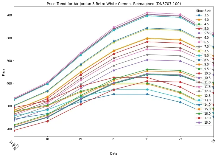

Price trend analysis can give us a lot of insights into the market. For example, we can see that the price of this particular shoe had a sharp increase bump.
Another thing we can see is that the price of some sizes deviates less than others - let's take a look at price volatility:

price_volatility = price_pivot_df.std()
price_volatility.plot.bar(figsize=(10, 6))
plt.title("Price Volatility for Each Shoe Size")
plt.xlabel("Shoe Size")
plt.ylabel("Standard Deviation")
plt.xticks(rotation=0)
plt.show()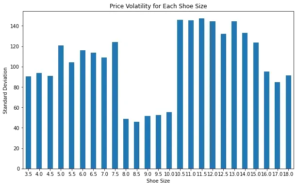

In this example, we can see that the prices of more common men's shoe sizes tend to be less volatile than the the more rare sizes. This is a good indicator that the market is more stable for the more common sizes because of higher trade volume.

To predict future pricing trends we can further create a price distribution trend chart:

price_pivot_df.plot.box(figsize=(12, 8))
plt.title("Price Distribution for Each Shoe Size")
plt.xlabel("Shoe Size")
plt.ylabel("Price")
plt.xticks(rotation=0)
plt.show()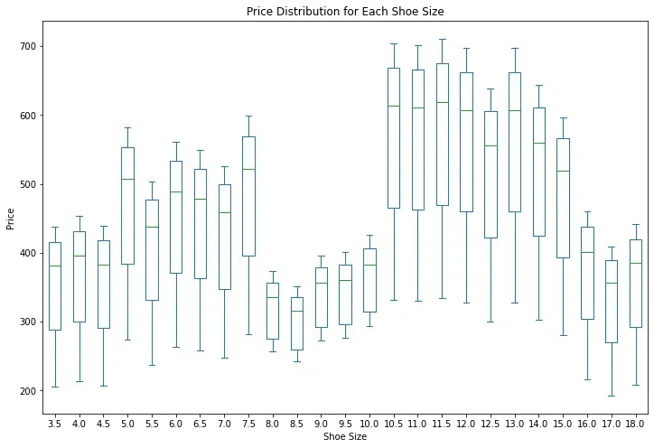

This is just a brief example of how easy it is to scrape and analyze footwear market data. We can use the same techniques to analyze other markets like clothing, accessories, and even collectible items.

Summary

In this quick overview, we've taken a look at how web scraping can be used to dive into footwear market analytics using basic Python analytic tools.

We used Goat.com to scrape Air Jordan 3 sneaker data and analyze the market distribution by product features (like shoe size and color). Then, we've taken a historical look at a single product's price trends we've scraped through out the week and saw that some shoe sizes are more volatile than others.

Web scraping is a great resource for market research and analytics as the web is full of free public data. Using Python and the existing web scraping and data analysis tools we can do a fair bit of market analytics using just few lines of code!